[Post 3 of 10 in the series examining how to build a daily fantasy model]

Welcome back to this series on building a DFS model for baseball. Hopefully you find this as timely as I do now that we’re less than 22 days out from the first spring training games, about 4 weeks from the World Baseball Classic, and just two months from the first pitch of the 2026 season.

So far in this series we’ve tackled two foundational things – what we are (and are not) building and setting up the environment. In this post we’re going to shift our focus and talk about the data itself – and really start building this tool.

The core data we’re going to use can be found in the pybaseball package. This package is a Python library that automates the collection of (among many other things) pitch-level data from sources like Baseball Savant and FanGraphs. This is what we’re going to use for building our model. Although we’ll walk through examples here, you will want to bookmark the pybaseball docs and Statcast CSV definitions so you have a handy reference for things.

A quick look through the Statcast CSV definitions will give you an idea of what kind of data we can pull from this library – and it’s tremendous. At a pitch-level, we can see not just the meta data about the situation (inning, team, batter, who’s on first, etc.) or the result of the pitch (ball, strike, home run, etc.) but where it crossed home plate, if it was hit what the estimated distance was, and how the outfield was aligned – among a ton of other stuff. I highly recommend checking it out.

But let’s go ahead and pull some of that data in.

In your first cell you should have your imports to load the appropriate libraries. Make sure you have the packages below loaded. Note that we’ve specifically called out “statcast” and “chadwick_register” as libraries within pybaseball. Technically we don’t have to do that – “import pybaseball” already covers that – but I have found it makes it easier to manage if I don’t have to prepend a “pybaseball.” to the front of a call to one of those two so I carve it out separately. I’m sure if a professional Python programmer saw my code they’d probably be able to refactor it to be faster, but my approach works for me. (for more information on that, check here)

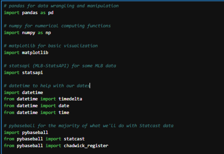
Also note I comment every material block of code. In some cases that’s every line; in other cases that’s a block of common lines. You do you, but it’s frustrating enough when you know what the code you wrote four months ago is supposed to be doing and it’s not doing it – imaging having to do it having no idea what it’s supposed to be doing because there aren’t any comments and the code looks foreign.

In statsapi there is a function called “schedule” that we can call to get the schedule of games within a specific date range. We can call that with:

start_date = datetime.date(2025, 9, 1)
end_date = datetime.date(2025, 9, 5)
schedule = statsapi.schedule(start_date=start_date , end_date=end_date)

We created two variables to hold our start and end dates, and then passed those to the statsapi “schedule” function. The results were returned into a list containing a dict[ionary] for each game. (how did I know what the data was returned as? The documentation.) Go ahead and run that code; it shouldn’t take too long since we’re only grabbing schedule data for five days’ worth of games.

Once it’s run we can examine the list we called “schedule” by running this code in a cell:

print(schedule)

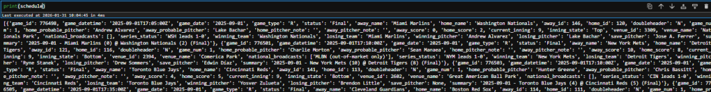
Pretty ugly and while not unreadable, pretty hard to read. So, we’re going to drop all that data into a pandas dataframe to make it easier not just to read but to do things with. Replace the “print(schedule)” code with this, which will take that data and turn it into a dataframe called “rawdata” and then give us the first 5 rows:

rawdata = pd.DataFrame(schedule)
rawdata.head(5)

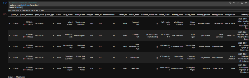
A much cleaner way to view it. We can’t see all the columns, though – note the elipses (“…”) in the middle between ‘doubleheader’ and ‘venue_id’. To fix that, add this code and run it. I usually put this code in its own “setup cell” right after I import package, but you can put it anywhere before you start showing dataframes and after you’ve imported pandas:

pd.set_option('display.max_columns', None)

Run that cell and it will tell pandas to show you all the columns in a dataframe. Then go back to your rawdata cell and re-run that; you should see all the columns appear.

Now we have a dataframe with five days’ worth of schedule data in it. Let’s move on and look at player data.

For this we’re going to use pybaseball; specifically the chadwick_register. To retrieve the Chadwick Register into a dataframe:

playersDF = chadwick_register()
playersDF.head(5)

You can see it’s pretty compact – but pretty powerful. It provides first and last names, various keys to use when matching with different sites, and when they played first and last in the majors.

We have schedules and players. Now let’s look at some actually Statcast data. This is a little different (but not much) than what we did with schedule data. Run this code:

pybaseball.cache.enable()

start_date_string = start_date.strftime("%Y-%m-%d")
end_date_string = end_date.strftime("%Y-%m-%d")

statcast_df = statcast(
start_dt= start_date_string,
end_dt= end_date_string
)

The first line turns on the cache function of pybaseball. If you’re pulling in more than a day’s worth of data (keep in mind, this is at the pitch level) I recommend this function call.

The rest is simply calling the “statcast” function from pybaseball and putting it in a dataframe we called ‘statcast_df’. The catch here is that we couldn’t simply pass it the variables we created for schedule data, so we had to manipulate them a bit. Instead of accepting a date variable (which is what “schedule” wanted), “statcast” is looking for a string representation of that date variable. So, we simply append a function to turn the date value into a string and pass that.

Clean? Not necessarily, but it works. Now let’s see the size of this data (5 days of pitch-level) and then use that .head() function on the dataframe to see what kind of data we’ve got:

print(statcast_df.shape)
statcast_df.head(15)

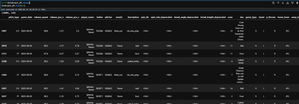
We can see at the very top of the output the shape (rows, columns) of the dataframe. It consists of 18,881 rows and 118 columns. That’s 2.2 million points of data for five days, or an average of 446 thousand every day. If you enjoy data this should excite you (and if you don’t like data, I am happy you’re here but a little curious why; drop me a comment!) – we’re going to have a lot of fun.

Before we wrap up this post and I turn you loose to play around with what you’ve just found, let’s add a little more context to the data. Right now we know who the pitcher is (that’s the ‘player_name’ field), and we can figure out the batter if we look in the ‘des’ field for an actual event (strikeout, ground out, walk, etc.). But let’s use that Chadwick Register data to augment this. Add this code in a cell after everything you’ve already done:

full_names = playersDF['name_first'] + ' ' + playersDF['name_last']
name_lookup = full_names.groupby(playersDF['key_mlbam']).first()

statcast_df['batter_name'] = statcast_df['batter'].map(name_lookup)
statcast_df['pitcher_name'] = statcast_df['pitcher'].map(name_lookup)

statcast_df.sample(10)

This is going to create a “full name” field and add that into the Statcast data where the ‘batter’ or ‘pitcher’ fields match the ‘key_mlbam’ field in the Chadwick Register data. The last line just takes a sample of 10 records (vs. head(10) which would be the first 10) so you can check the data and see what it shows. Those new columns should be on the right.

Have fun with the Statcast data; in the next post we’re going to start turning this data into something useful by adding some field as well as trimming the size of the dataset to make it more manageable.

---

Affiliate Disclosure: I’m a big fan of transparency, so I want to make sure you know that on this site you may find certain links to products or services that I’m an affiliate of. This means I may make a commission for any purchases you make using those links. If you are not comfortable with that that’s completely fine – you can feel free to find the same product or service other ways and it won’t hurt my feelings. I keep my affiliate links minimal and use them only as an opportunity to help offset costs while helping others.

Affiliate links:
DailyGrind. Daily fantasy sports predictions.
OddsShopper. Betting optimization tool.